


When we look at graphs (or trees), we often see this nice collection of nodes with the entire structure fully mapped out:
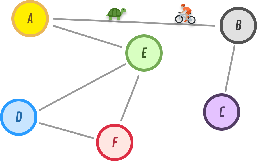
In real-world scenarios, this fully mapped-out view is the final result of our code having fully explored the graph. When we encounter a graph for the first time, this is what our computers see:
It is a blank unknown slate. We have to actively explore our graph node-by-node to create the final picture of what all the nodes and edges look like. There is an art and science to how we perform this exploration. That’s where the stars of this tutorial, Depth-First Search (DFS) and Breadth-First Search (BFS), come in. In the following sections, we’ll learn how they work to help us fully explore a graph.
For a comprehensive and beginner-friendly look at data structures and algorithms, check out Kirupa's best-selling book on this topic.
Both Depth-First Search (DFS) and Breadth-First Search (BFS) are two approaches used to explore a graph. We’ll get into the nitty-gritty details of how they work, but let’s keep it high-level right now. Imagine we have a map with different locations, as shown below:
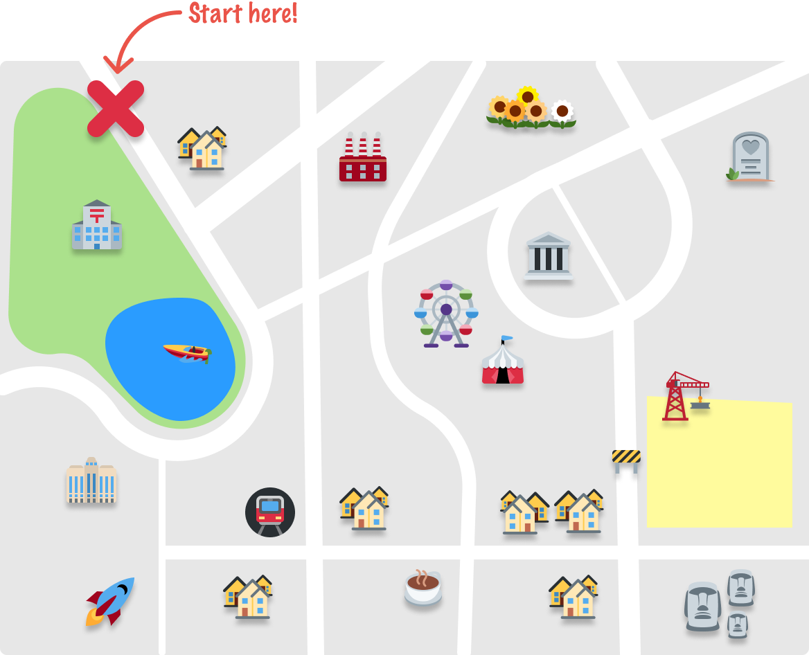
Our goal is to start from our starting point and explore all of the places. We’ll do this exploring using both a DFS approach and a BFS approach. By the end of this, we’ll be able to clearly see how these two approaches differ!
DFS is like exploring the map by picking one location and going as far as possible along a single path before backtracking and trying another path:
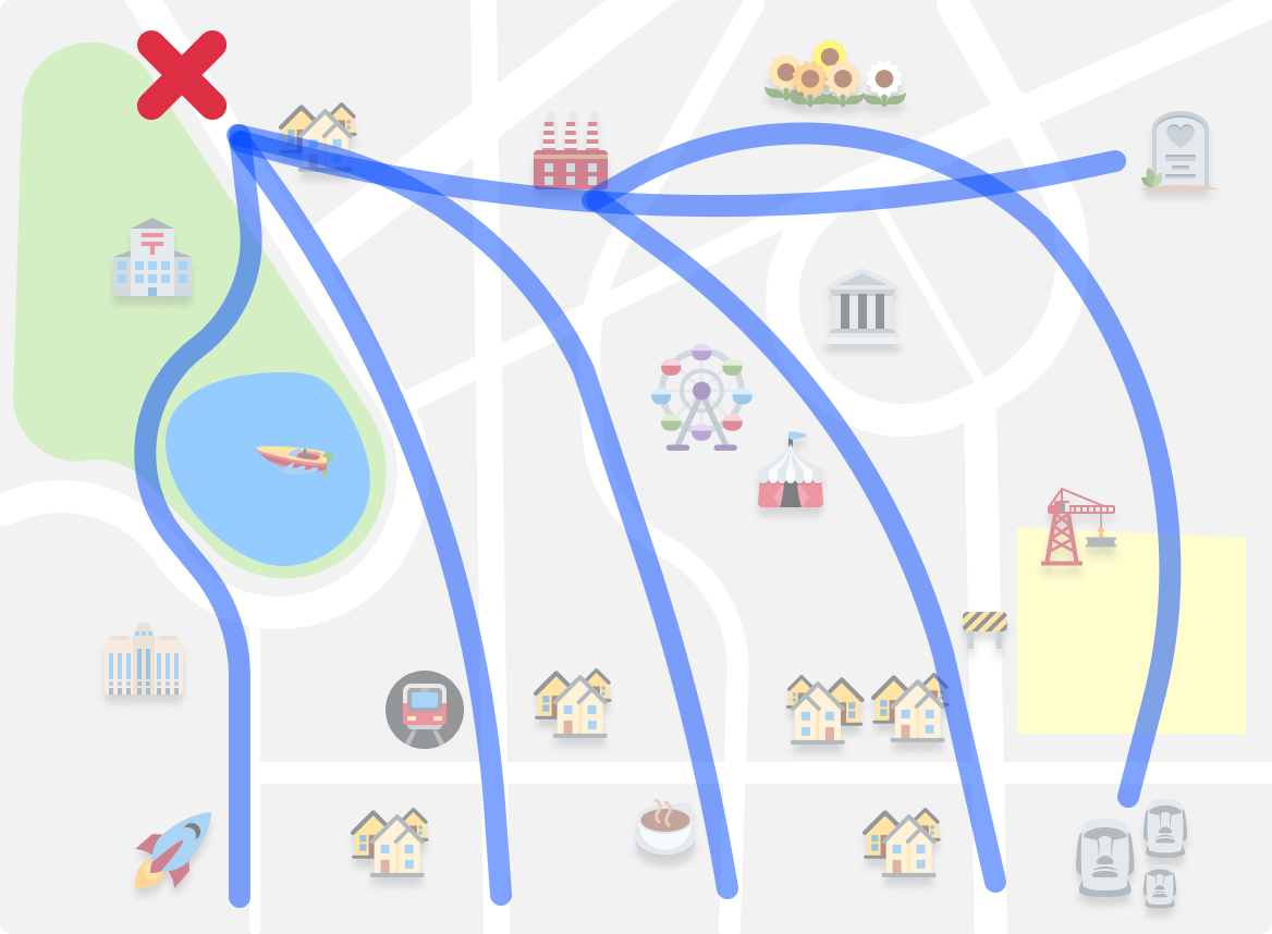
It's like taking one road and following it until we can't go any further, then going back and trying a different road. We keep doing this until we have explored all possible paths.
On the other hand, BFS is like exploring the map by starting at one location and gradually moving outwards:
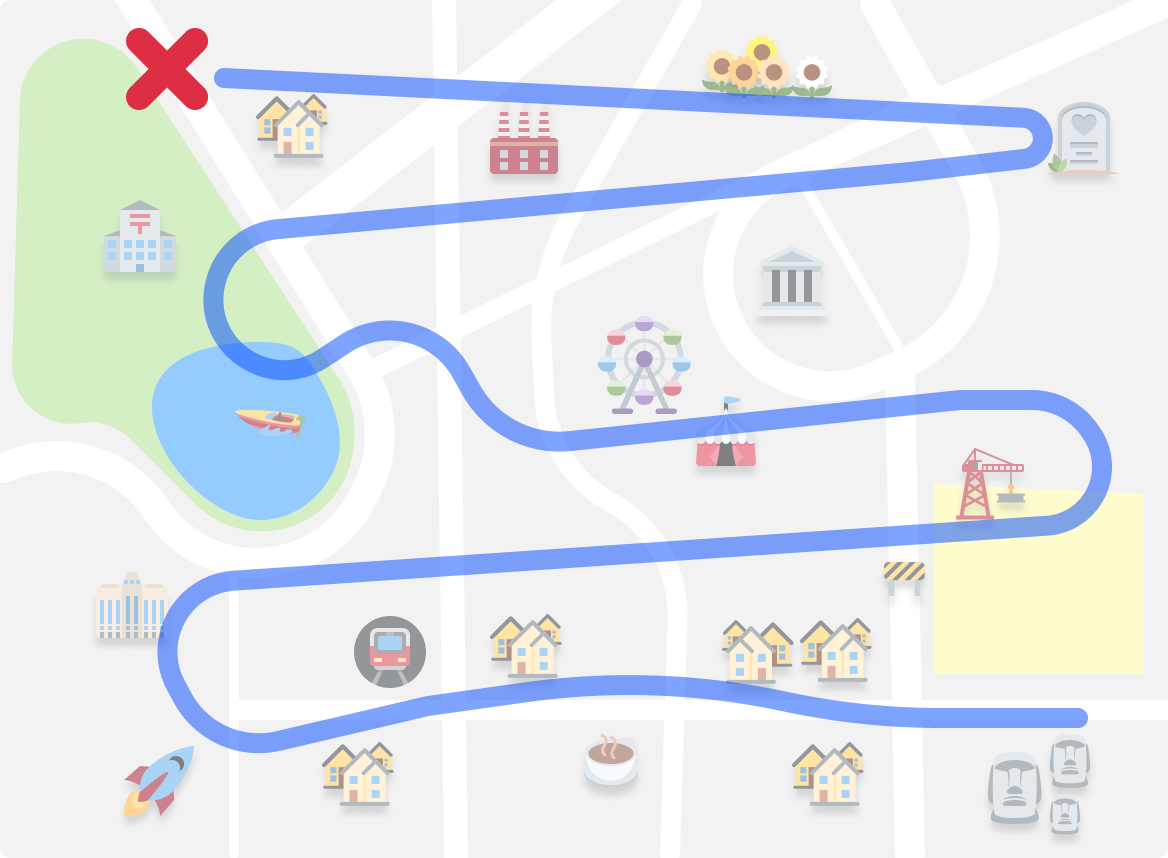
It's similar to how we might search for something by checking all the places in our immediate neighborhood first before expanding our search to other places.
As you can see, the end result of using either DFS or BFS is that we explore all the interesting landmarks. The gigantic detail lies in how we did this exploration. Both DFS and BFS are quite different here, and we’ll go beyond the generalities and get more specific about how they both work in the next section.
To more deeply understand how Depth-First Search (DFS) and Breadth-First Search (BFS) work, let’s work with a more realistic graph example. Our example graph will look as follows:
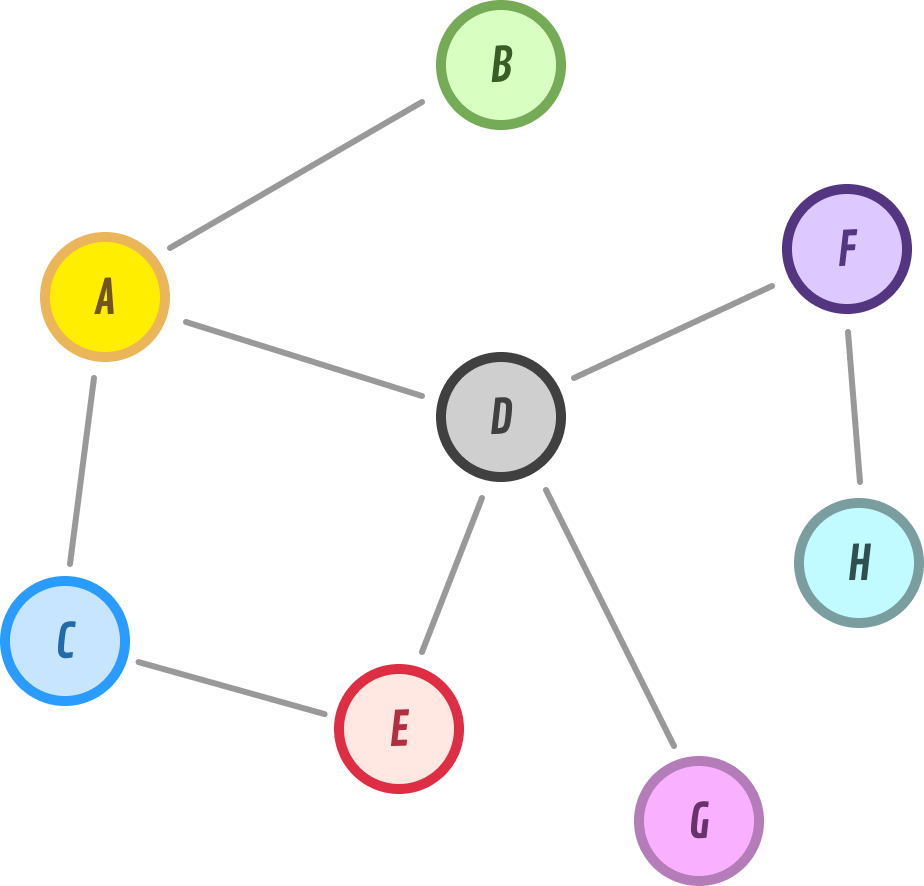
This graph is fairly plain. It is undirected, cyclic, and contains a bunch of nodes. In the following sections, we’ll walk through how we’re going to explore all of the nodes contained here.
DFS works by starting at a chosen node and then exploring as far as possible along each branch before hitting a dead end, backing up (aka backtracking), and trying again with the next unexplored node. It’s example time.
With graphs, we can start exploring from any arbitrary node. To keep things simple, we are going to start with node A:
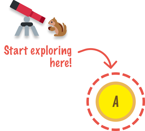
Let’s take a quick time out and call out two things here:
Getting back to it, we are at node A, and we are going to explore it. This leads us to discover nodes B, C, and D:
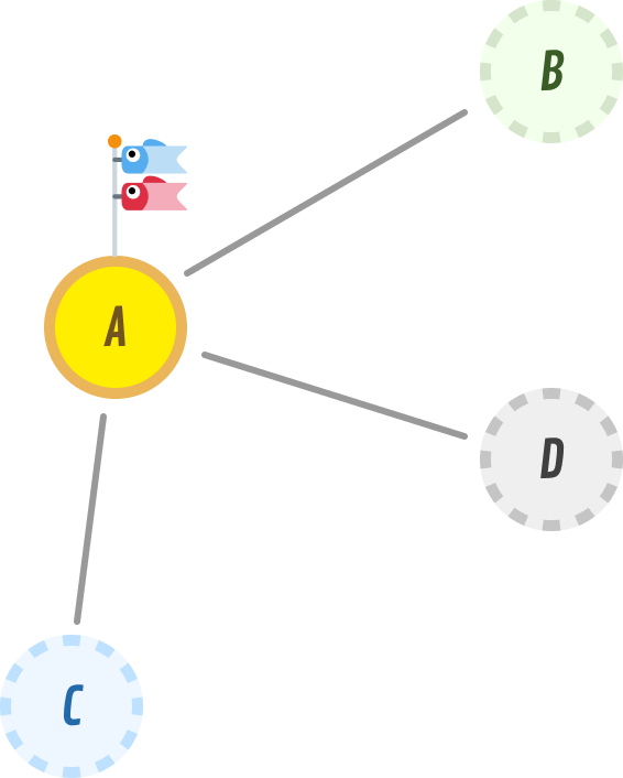
We can keep track of our findings by using the same explored and discovered terminology we used earlier when looking at how to traverse binary trees:
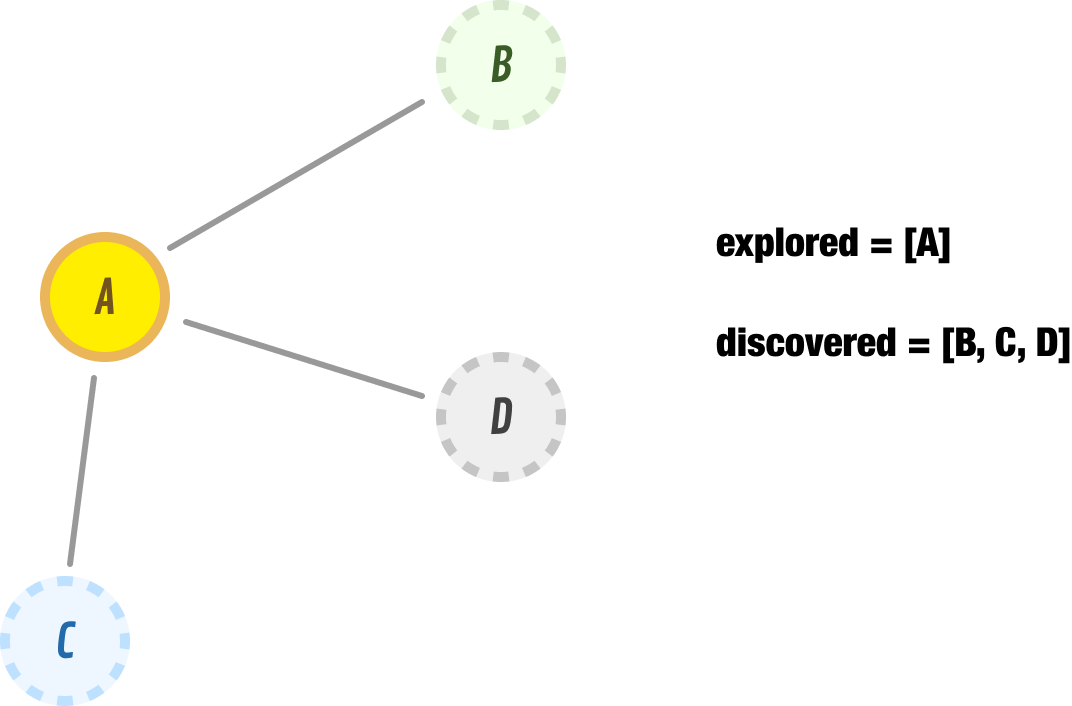
As of right now, our explored list is node A. The discovered list is nodes B, C, and D.
Next, we explore the first item in our discovered list. This would be node B. When we explore node B, we find that it has node A as a neighbor. Since A is a node we have already explored, we don’t consider that to be a new node that we have discovered.
For what we are concerned about, node B has no new neighbors. We remove node B from our discovered list and move it over to our explored list:
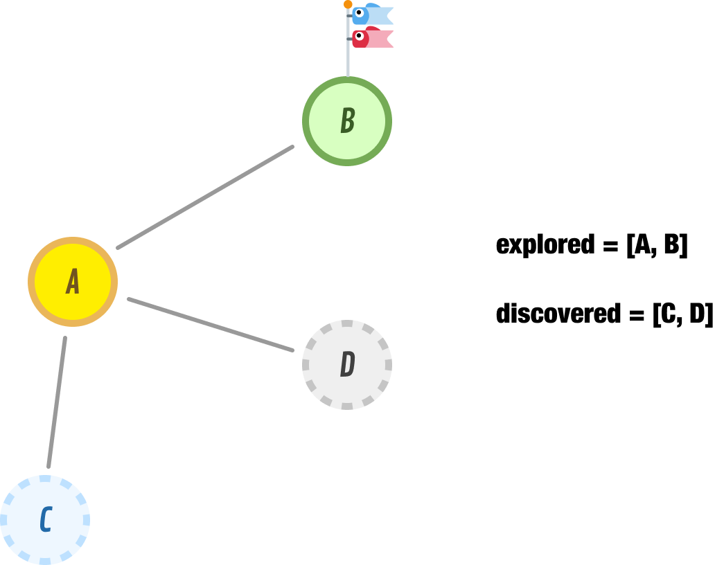
Because we reached a dead-end with B, we backtrack by retracing our steps and exploring the next nearest unexplored node, which is represented in our discovered list as node C. When we explore node C, we find that it has nodes A and E as its neighbors. Because node A has already been explored, the only new addition to our discovered list is node E. We move node C from our discovered list to our explored list, and we add node E node to the front of our discovered list:
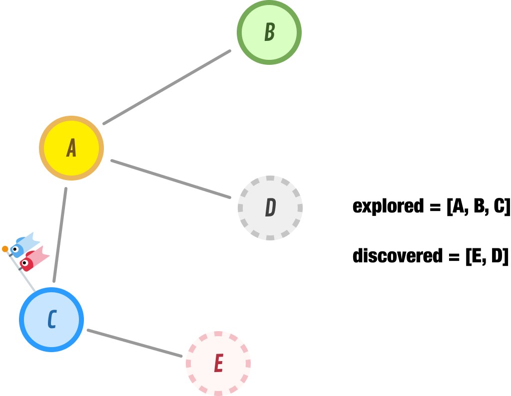
Note that we didn’t add node E to the end of our discovered list. We added it to the front, and this ensures that this is the node we explore next. This is an important implementation detail of the DFS approach that we should keep in mind.
When we explore node E, nodes D and C show up as neighbors. Node C is one we have already explored, and node D is already in our list to be discovered next. This puts us in the following state:
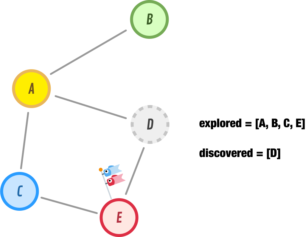
Because we don’t have any new nodes to discover, we go ahead and explore node D next. When we explore node D, we discover nodes F and G as new nodes to explore in the future. Node E, since we already explored it, is happily ignored:
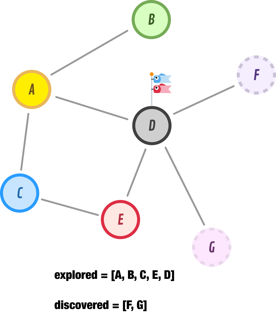
If we speed things up a bit and continue the logic we have employed so far, we will explore node F next. Node F has one unexplored node, and that is node H:
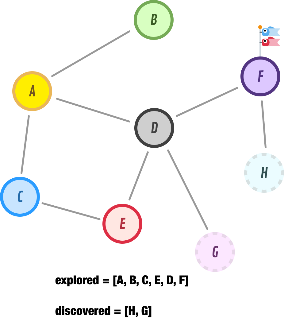
After moving node F to our explored list, we add node H to the beginning of our discovered list and go exploring it next:
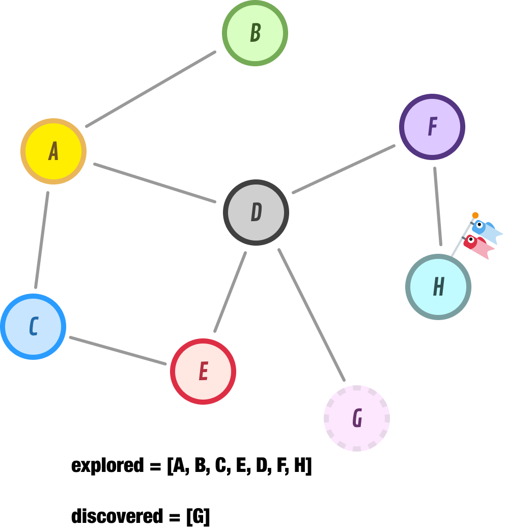
Node H has no neighbors, so we backtrack to the next unexplored node which is. lucky node G:
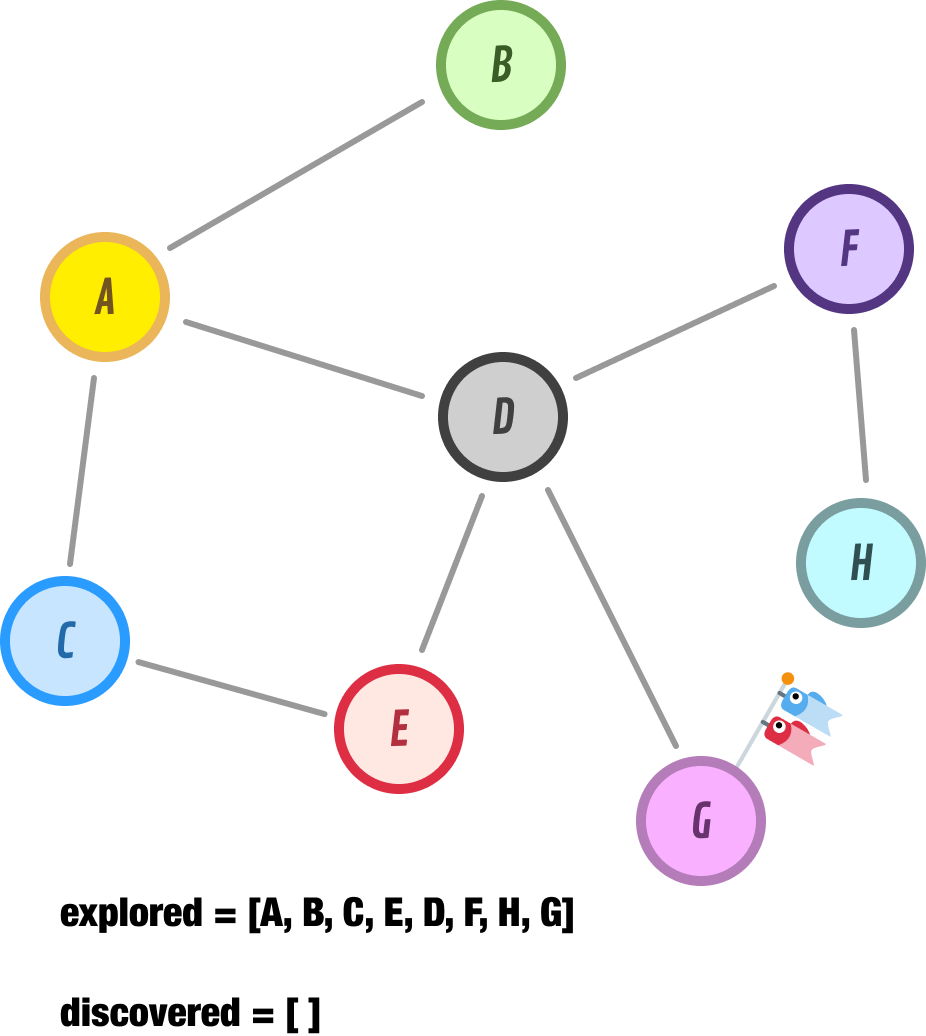
Node G has no neighbors. At this point, we have no more nodes to explore further. Our discovered list is empty. When we run into this situation, we can safely say that we have fully explored the reachable parts of our graph. The path our DFS approach took to discover all of our nodes is captured by our explored list, and it is A-B-C-E-D-F-H-G.
In a BFS approach, we start at a given node, explore all of this node’s neighbors, and then move on to the next level of nodes. It’s very different than what we saw with DFS earlier, and these differences will be clear as we walk through our example.
We are going to start our exploration from node A:
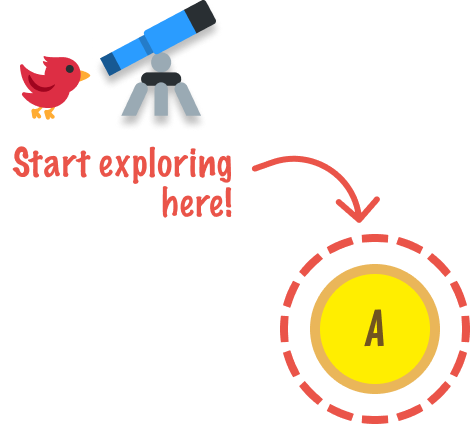
The first thing we do is discover if node A has any neighbors. As it turns out, it does:

Node A has three neighbors, and we go ahead and catalog them in our discovered list for exploration later. The next node we are going to explore is the first node under our discovered list, and that is node B. Node B has no neighbors, so we go ahead and move it from our discovered list and move it into our explored list:

So far, what we’ve seen in our early exploration closely mimics what we saw with DFS earlier. That will all be changing momentarily.
The next node we are going to explore is node C. Node C has one neighbor, and that is node E:
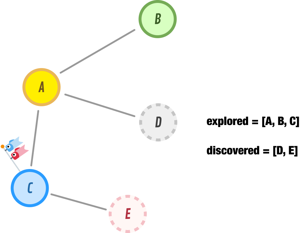
Because we have explored node C, we move it from the discovered list to our explored list. We then add our newly discovered node E to our discovered list. Notice where we add it. We don’t add it to the front of our list like we did with DFS earlier. Nope. We add it to the end of our discovered list. Any newly discovered nodes in a BFS approach will always be appended at the end. This ensures that nodes we had discovered earlier remain at a higher priority for being explored next.
This leads us to the next node we are about to explore, and that is node D. Node D has two neighbors, nodes F and G:
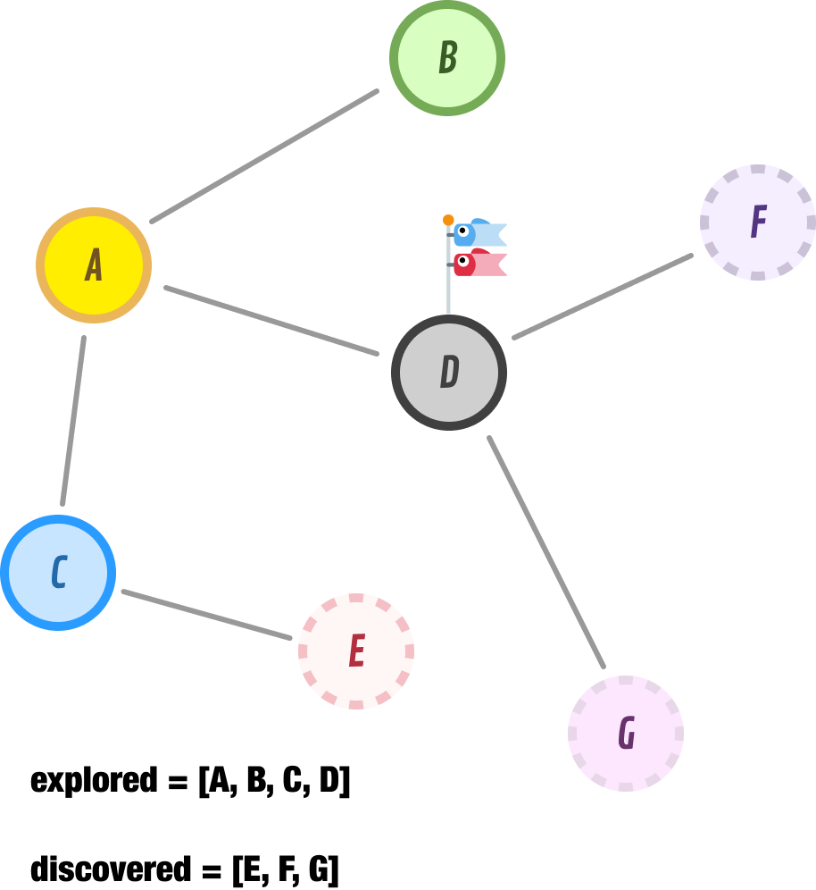
At this point, Node D moves into the explored list, and our discovered list now contains nodes E, F, and G.
The next node we explore is node E:
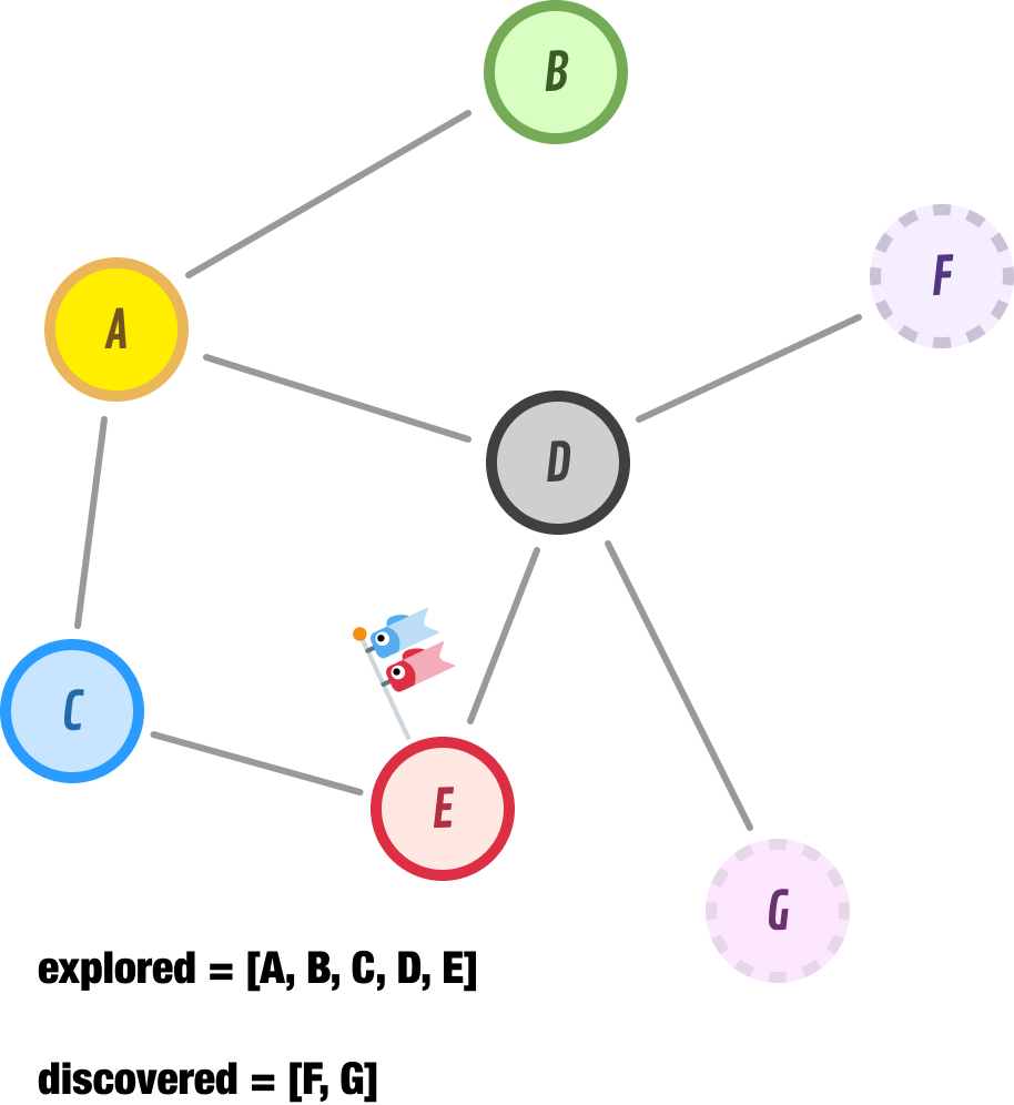
Node E doesn’t have any new unexplored neighbors, so we just move it to our explored list and move on. Let’s go a bit faster here.
The next node to explore is node F, and it has nodes D and H as its neighbors:
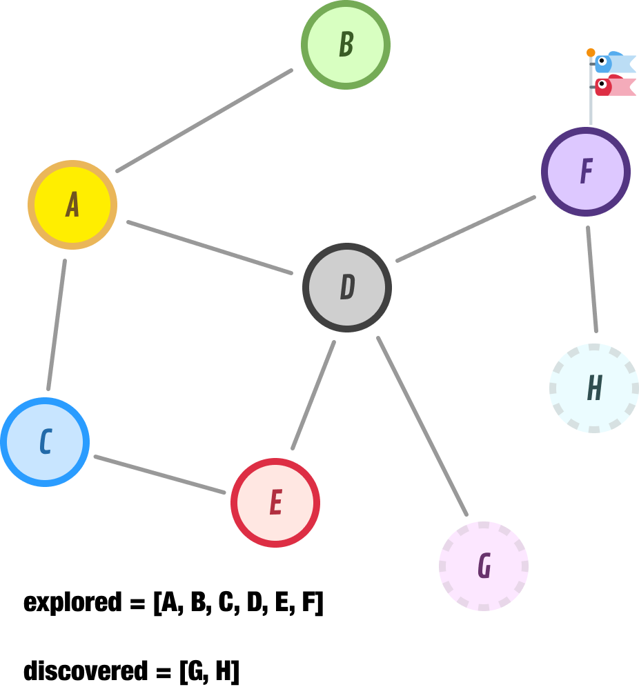
Node D has already been explored, but node H is new. Let’s add it to the end of our discovered list and move on to Node G:
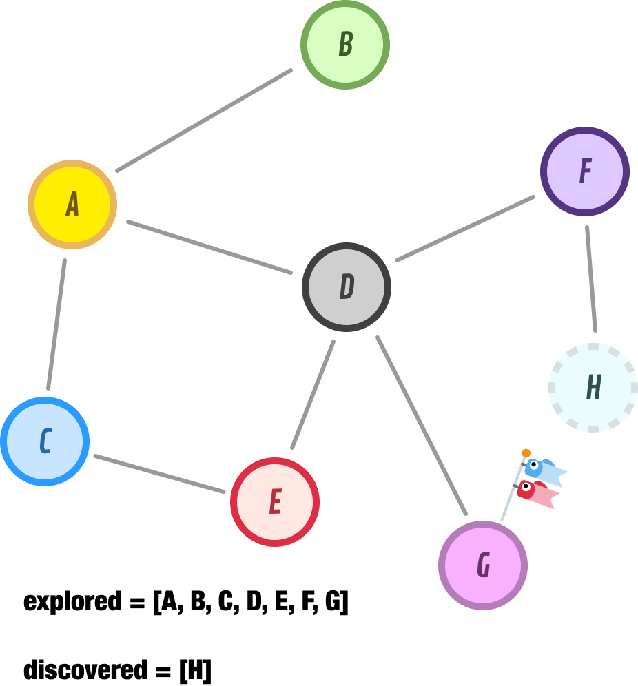
Node G has no unexplored neighbors, so we tag it as explored and move on to node H:
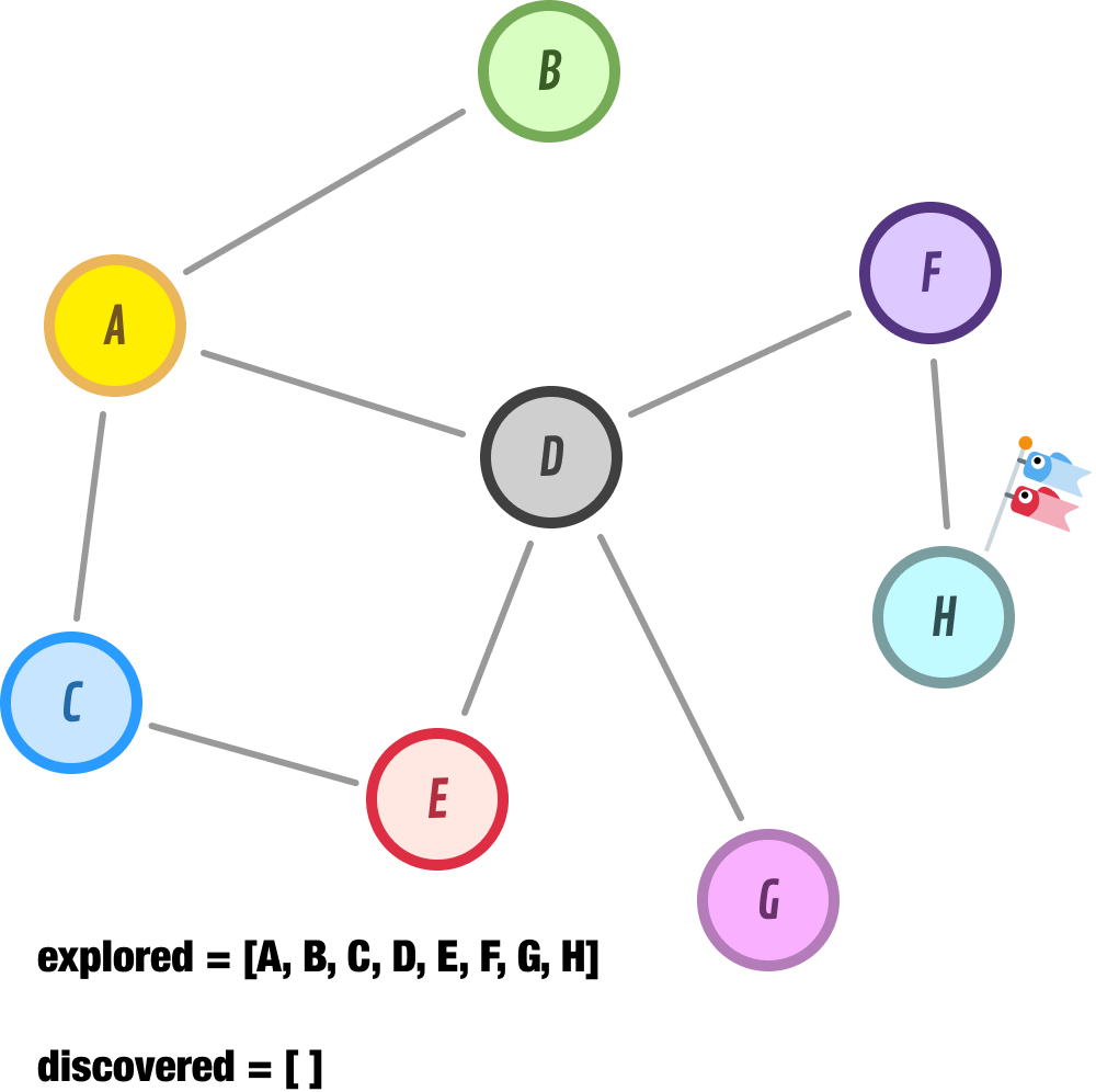
Node H has no new unexplored neighbors, so we go ahead and move it to our explored list. At this point, our discovered list is empty, and we have no more nodes left to discover. The explored list tracks the order our BFS approach took for exploring all of our nodes, and that order is A-B-C-D-E-F-G-H.
We have seen two approaches for exploring all the connected nodes in a graph. We started off by looking at Depth-First Search (DFS) and its way of exploring nodes by going as deep as possible along each branch before backtracking:
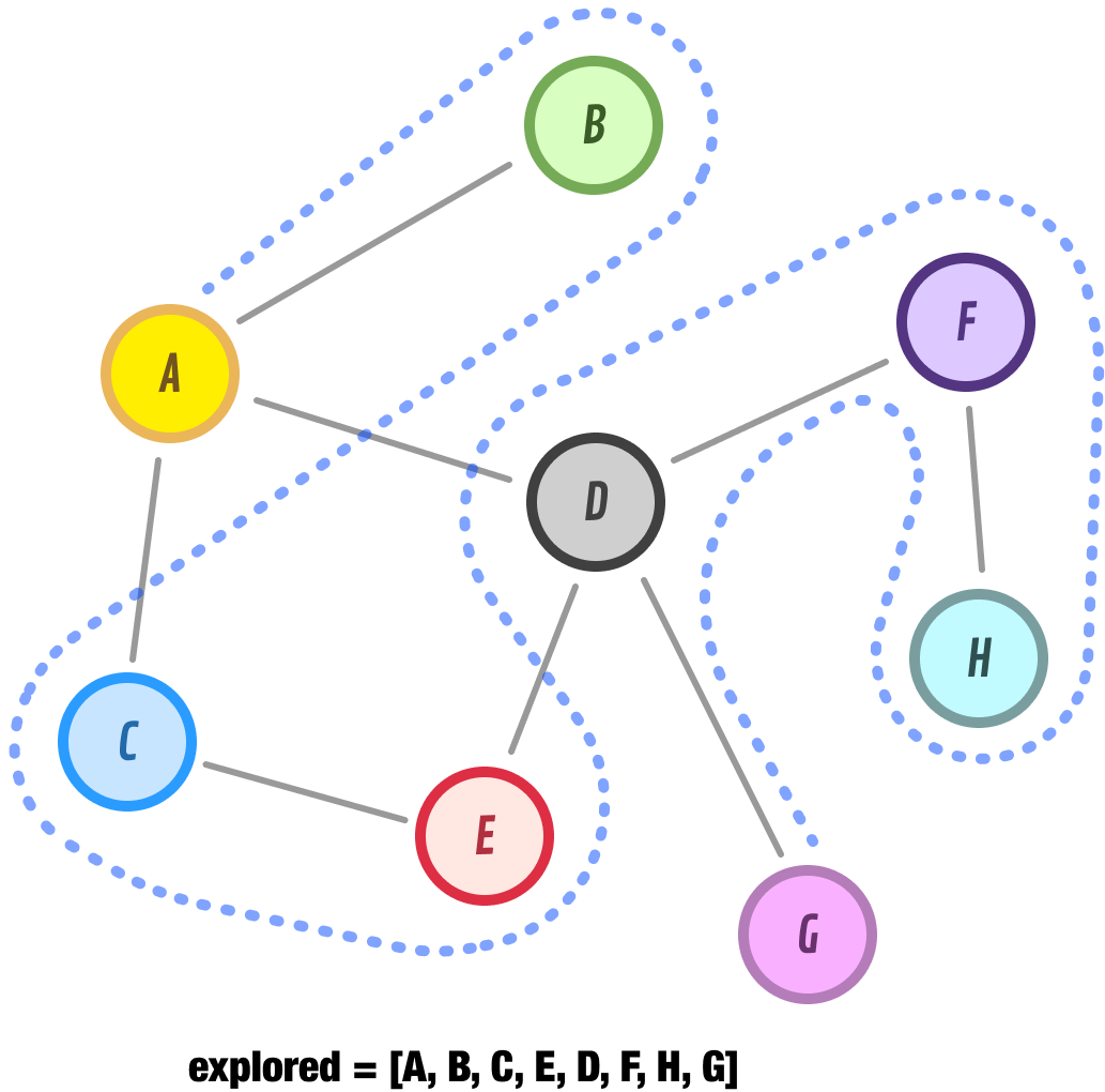
The second approach is Breadth-First Search (BFS), which explores nodes level by level, starting from the initial node and moving outward, visiting all the neighbors before moving to the next level:
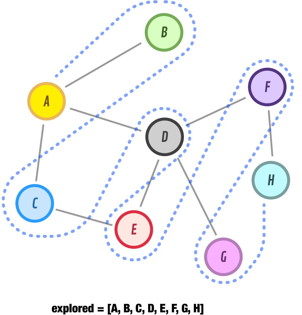
These two approaches for exploring nodes lead to the following state:
Depending what our purpose is for exploring our graph, we’ll use either DFS or BFS. If we are looking for just a way to explore all the nodes in a graph, then pick between DFS or BFS randomly. You can’t go wrong with either.
Now that we have seen in great detail how DFS and BFS work to explore the nodes in a graph, let’s shift gears and look at how both of these exploration approaches are implemented. We are going to be building on top of the Graph class we looked at earlier when looking specifically at the Graph data structure, so what you are about to see will be a lot of code that is familiar with some new code (that is highlighted) that implements what we need to to have DFS and BFS:
class Graph < constructor() < // Map to store nodes and their adjacent nodes this.nodes = new Map(); // Flag to indicate if the graph is directed or undirected this.isDirected = false; >// Add a new node to the graph addNode(node) < if (!this.nodes.has(node)) < this.nodes.set(node, new Set()); >> // Add an edge between two nodes addEdge(node1, node2) < // Check if the nodes exist if (!this.nodes.has(node1) || !this.nodes.has(node2)) < throw new Error('Nodes do not exist in the graph.'); >// Add edge between node1 and node2 this.nodes.get(node1).add(node2); // If the graph is undirected, add edge in the opposite direction as well if (!this.isDirected) < this.nodes.get(node2).add(node1); >> // Remove a node and all its incident edges from the graph removeNode(node) < if (this.nodes.has(node)) < // Remove the node and its edges from the graph this.nodes.delete(node); // Remove any incident edges in other nodes for (const [node, adjacentNodes] of this.nodes) < adjacentNodes.delete(node); >> > // Remove an edge between two nodes removeEdge(node1, node2) < if (this.nodes.has(node1) && this.nodes.has(node2)) < // Remove edge between node1 and node2 this.nodes.get(node1).delete(node2); // If the graph is undirected, remove edge in the opposite direction as well if (!this.isDirected) < this.nodes.get(node2).delete(node1); >> > // Check if an edge exists between two nodes hasEdge(node1, node2) < if (this.nodes.has(node1) && this.nodes.has(node2)) < return this.nodes.get(node1).has(node2); >return false; > // Get the adjacent nodes of a given node getNeighbors(node) < if (this.nodes.has(node)) < return Array.from(this.nodes.get(node)); >return []; > // Get all nodes in the graph getAllNodes() < return Array.from(this.nodes.keys()); >// Set the graph as directed setDirected() < this.isDirected = true; >// Set the graph as undirected setUndirected() < this.isDirected = false; >// Check if the graph is directed isGraphDirected() < return this.isDirected; >// Class variable for storing explored nodes #explored = new Set(); getExploredNodes() < return this.#explored; >// // Depth First Search (DFS) // dfs(startingNode) < // Reset to keep track of explored nodes this.#explored = new Set(); // Call the recursive helper function to start DFS this.#dfsHelper(startingNode); >#dfsHelper(node) < // Mark the current node as explored this.#explored.add(node); // Get neighbors to explore in the future const neighbors = this.getNeighbors(node); for (const neighbor of neighbors) < if (!this.#explored.has(neighbor)) < // Recursively call the helper function for unexplored neighbors this.#dfsHelper(neighbor); >> > // // Breadth First Search (BFS) // bfs(startingNode) < // Reset to keep track of explored nodes this.#explored = new Set(); // Queue to store nodes to be explored const queue = new Queue(); // Mark the starting node as explored this.#explored.add(startingNode); // Enqueue the starting node queue.enqueue(startingNode); while (queue.length >0) < // Dequeue a node from the queue const node = queue.dequeue(); const neighbors = this.getNeighbors(node); for (const neighbor of neighbors) < if (!this.#explored.has(neighbor)) < // Mark the neighbor as explored this.#explored.add(neighbor); // Enqueue the neighbor to be explored queue.enqueue(neighbor); >> > > >This uses an implementation of a queue from our Queues in JavaScript article. You can either copy/paste the implementation from that article or reference it directly via the following script tag:
We can certainly modify this code to avoid using a queue and work with arrays directly, but the performance penalties may be quite high - especially if we are dealing with a lot of nodes.
The new additions to our earlier Graph implementation are the dfs , #dfsHelper , getExploredNodes , and bfs methods along with a few private variables. To perform an exploration, we need to call the appropriate dfs or bfs method with a starting node provided as the argument. Take a look at the following code, where we re-created the graph we looked at in the previous sections and perform both a DFS and BFS operation on it:
// Our graph from earlier! const graph = new Graph(); graph.addNode("A"); graph.addNode("B"); graph.addNode("C"); graph.addNode("D"); graph.addNode("E"); graph.addNode("F"); graph.addNode("G"); graph.addNode("H"); graph.addEdge("A", "B"); graph.addEdge("A", "C"); graph.addEdge("A", "D"); graph.addEdge("C", "E"); graph.addEdge("D", "E"); graph.addEdge("D", "F"); graph.addEdge("D", "G"); graph.addEdge("F", "H"); console.log("DFS:"); graph.dfs("A"); // Perform DFS starting from node "A" console.log(graph.getExploredNodes()); console.log("BFS:"); graph.bfs("A"); // Perform BFS starting from node "A" console.log(graph.getExploredNodes());When you run this code, pay attention to the console output where we print the final explored node for both our DFS approach and BFS approach. Notice that the output matches what we manually walked through in the previous sections.
When walking through how DFS and BFS work, a key distinction was in where in our discovered list newly discovered nodes get added.
For DFS, newly discovered items are added to the beginning of our discovered list. This ensures DFS maintains its behavior where it explores deep into a path. For BFS, newly discovered items are added to the end of our discovered list. This behavior ensures BFS fully explores its immediate neighbors first before going to the next level.
Our implementations of DFS and BFS reflect the differing behavior on how discovered items are added to our discovered list. For DFS, we perform a recursive call on the newly discovered node:
for (const neighbor of neighbors) < if (!explored.has(neighbor)) < // Recursively call the helper function for unexplored neighbors this.#dfsHelper(neighbor, explored); >>This allows us to mimic a stack-like behavior by relying on our underlying runtime’s call stack to preserve the order of nodes to explore.
With BFS, we implement a Queue to keep track of our discovered nodes:
for (const neighbor of neighbors) < if (!explored.has(neighbor)) < // Mark the neighbor as explored explored.add(neighbor); // Enqueue the neighbor to be explored queue.enqueue(neighbor); >>This allows us to efficiently add items to the end and remove items from the beginning to explore more deeply.
There is one more thing before we wrap things up here, and that has to do with how efficient both DFS and BFS are when it comes to exploring a graph.
In the grand scheme of things, if we had to summarize the performance, it is safe to say that both DFS and BFS run in linear time and take up a linear amount of space. That’s not too shabby.
Well, this was quite a blast! In the many preceding sections, we learned how to explore all the nodes in a graph using both Depth-First Search (DFS) and Breadth-First Search (BFS)! On the surface, both DFS and BFS are similar. You throw a starting node at them and a graph to start exploring. Both approaches will explore all the nodes that they encounter. What sets them apart is how they go about doing their exploration. DFS goes deep down the first path it finds and doesn’t stop until it reaches a dead-end, at which point it goes back to last unexplored node and continues diving deep again. BFS goes broad. It explores all its immediate nodes first and then goes to the next level and explores all of those nodes next. It takes a gradual outward approach.
In the end, by learning DFS and BFS, we gain valuable tools to tackle a wide range of graph problems. As we may find out shortly, DFS and BFS are one of the more foundational pieces of path-finding algorithms and other more interesting things we will want to do with graphs. Happy exploring!
Just a final word before we wrap up. If you have a question and/or want to be part of a friendly, collaborative community of over 220k other developers like yourself, post on the forums for a quick response!